Faster R-CNN最突出的贡献就在于提出了Region Proposal Network(RPN)代替了Selective Search,从而将候选区域提取的时间开销几乎降为0(2s -> 0.01s)
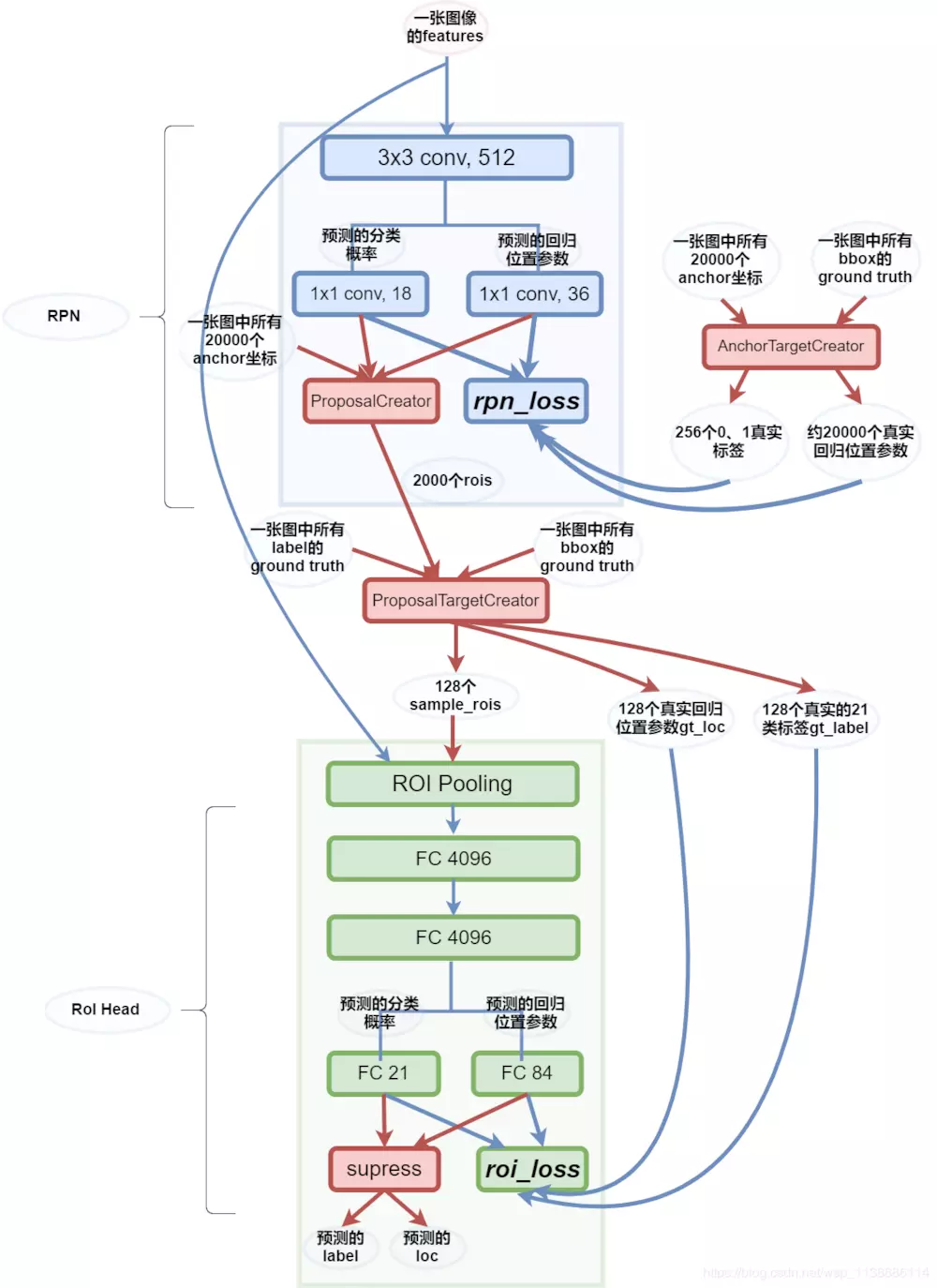
一切都要从一张图的特征开始说起:features。
RPN 接到features后,先做了一次3x3的卷积,再由两个1x1卷积操作分别得到分类score:2x9与位置偏移loc:4x9结构,这两个结构都会被ProposalCreator与rpn_loss所使用。
AnchorTargetCreator 用box与anchor联合得到拟合目标:loc与label。这里前景与背景的label总数为256,loc图外的标记为-1。
RPN_LOSS 将会利用上述预测信息与标签信息计算loss,以此来调整使得RPN网络预测的score与loc更好。只对前景计算回归损失。
ProposalCreator 的任务是拿到score与loc后,将loc转为roi,按照分数筛选先取12000,再通过极大值抑制去除重叠后再按照score选取前2000个roi。
ProposalTargetCreator 将ProposalCreator中得到的2000个roi与标签box利用ROU再进行筛选,留下正负样本共128个。
ROI Pooling 层得到这128个rois后,对其坐标对应到特征图,size缩小为1/stride(1/16)。这里在对应的时候,会存在无法整除的现象,所以后来又提出了ROI Align。对应好之后,还要对roi 实施Pooling操作,使得对应好的roi特征图池化到后面层能处理的大小(7x7),在这里还是有量化损失。
FC 21与FC 84 分别得到20+1(背景)类的分类与目标的位置。得到的数据将会与ProposalTargetCreator 中的真实标签计算roi_loss 。
名词解释:
t ∗ t_* t ∗ t x , t y t_x,t_y t x , t y t w , t h t_w,t_h t w , t h
t x = ( G x − P x ) / P w , ( 6 ) t y = ( G y − P y ) / P h , ( 7 ) t w = log ( G w / P w ) , ( 8 ) t h = log ( G h / P h ) , ( 9 ) \begin{array}{c}{t_{x}=\left(G_{x}-P_{x}\right) / P_{w},(6)} \\ {t_{y}=\left(G_{y}-P_{y}\right) / P_{h},(7)} \\ {t_{w}=\log \left(G_{w} / P_{w}\right),(8)} \\ {t_{h}=\log \left(G_{h} / P_{h}\right),(9)}\end{array}
t x = ( G x − P x ) / P w , ( 6 ) t y = ( G y − P y ) / P h , ( 7 ) t w = log ( G w / P w ) , ( 8 ) t h = log ( G h / P h ) , ( 9 )
目标函数为:
d ∗ ( P ) = w ∗ T Φ 5 ( P ) d_{*}(P)=w_{*}^{T}\Phi_{5}(P)
d ∗ ( P ) = w ∗ T Φ 5 ( P )
其中Φ 5 ( P ) \Phi_{5}(P) Φ 5 ( P ) w ∗ w_* w ∗ d ∗ ( P ) d_{*}(P) d ∗ ( P ) t ∗ t_* t ∗ d ∗ ( P ) d_*(P) d ∗ ( P )
L o s s = ∑ i N ( t ∗ i − w ^ ∗ T ϕ 5 ( P i ) ) 2 Loss=\sum_{i}^{N}(t_{*}^{i}-\hat{w}_{*}^{T}\phi_{5}(P^{i}))^{2}
L o s s = i ∑ N ( t ∗ i − w ^ ∗ T ϕ 5 ( P i ) ) 2
函数优化目标:
W ∗ = argmin w ∗ ∑ i N ( t ∗ i − w ^ ∗ T ϕ 5 ( P i ) ) 2 + λ ∥ w ^ ∗ ∥ 2 W_{*}=\operatorname{argmin}_{w_{*}}\sum_{i}^{N}\left(t_{*}^{i}-\hat{w}_{*}^{T}\phi_{5}\left(P^{i}\right)\right)^{2}+\lambda\left\|\hat{w}_{*}\right\|^{2}
W ∗ = a r g m i n w ∗ i ∑ N ( t ∗ i − w ^ ∗ T ϕ 5 ( P i ) ) 2 + λ ∥ w ^ ∗ ∥ 2
为什么t x , t y t_x,t_y t x , t y
为什么t w , t h t_w,t_h t w , t h
线性函数拟合非线性函数: lim x = 0 log ( 1 + x ) = x \lim _{x=0} \log (1+x)=x lim x = 0 log ( 1 + x ) = x
t w = log ( G w / P w ) = log ( G w + P w − P w P w ) = log ( 1 + G w − P w P w ) t_{w}=\log \left(G_{w} / P_{w}\right)=\log \left(\frac{G_{w}+P_{w}-P_{w}}{P_{w}}\right)=\log \left(1+\frac{G_{w}-P_{w}}{P_{w} }\right)
t w = log ( G w / P w ) = log ( P w G w + P w − P w ) = log ( 1 + P w G w − P w )
可以看到,当G w − P w = 0 G_w-P_w=0 G w − P w = 0
1
2
3
4
5
6
7
8
9
10
11
12
13
14
15
16
17
18
19
20
21
22
23
24
25
26
27
28
29
30
31
32
33
import numpy as np def compute_iou(box1, box2, wh=False): """ compute the iou of two boxes. Args: box1, box2: [xmin, ymin, xmax, ymax] (wh=False) or [xcenter, ycenter, w, h] (wh=True) wh: the format of coordinate. Return: iou: iou of box1 and box2. """ if wh == False: xmin1, ymin1, xmax1, ymax1 = box1 xmin2, ymin2, xmax2, ymax2 = box2 else: xmin1, ymin1 = int(box1[0]-box1[2]/2.0), int(box1[1]-box1[3]/2.0) xmax1, ymax1 = int(box1[0]+box1[2]/2.0), int(box1[1]+box1[3]/2.0) xmin2, ymin2 = int(box2[0]-box2[2]/2.0), int(box2[1]-box2[3]/2.0) xmax2, ymax2 = int(box2[0]+box2[2]/2.0), int(box2[1]+box2[3]/2.0) ## 获取矩形框交集对应的左上角和右下角的坐标(intersection) xx1 = np.max([xmin1, xmin2]) yy1 = np.max([ymin1, ymin2]) xx2 = np.min([xmax1, xmax2]) yy2 = np.min([ymax1, ymax2]) ## 计算两个矩形框面积 area1 = (xmax1-xmin1) * (ymax1-ymin1) area2 = (xmax2-xmin2) * (ymax2-ymin2) inter_area = (np.max([0, xx2-xx1])) * (np.max([0, yy2-yy1])) #计算交集面积 iou = inter_area / (area1+area2-inter_area+1e-6) #计算交并比 return iou
1
2
3
4
5
for object in all objects: (1) 获取当前目标类别下所有bbx的信息 (2) 将bbx按照confidence从高到低排序,并记录当前confidence最大的bbx (3) 计算最大confidence对应的bbx与剩下所有的bbx的IOU,移除所有大于IOU阈值的bbx (4) 对剩下的bbx,循环执行(2)和(3)直到所有的bbx均满足要求(即不能再移除bbx)
NMS是对所有的类别分别执行的。举个栗子,假设最后预测出的矩形框有2类(分别为cup, pen),在NMS之前,每个类别可能都会有不只一个bbx被预测出来,这个时候我们需要对这两个类别分别执行一次NMS过程。
1
2
3
4
5
6
7
8
9
10
11
12
13
14
15
16
17
18
19
20
21
22
23
24
25
26
27
28
29
30
31
32
33
34
35
36
37
38
39
40
41
42
43
44
45
import numpy as np class Bounding_box: def __init__(self, x1, y1, x2, y2, score): self.x1 = x1 self.y1 = y1 self.x2 = x2 self.y2 = y2 self.score = score def get_iou(boxa, boxb): max_x = max(boxa.x1, boxb.x1) max_y = max(boxa.y1, boxb.y1) min_x = min(boxa.x2, boxb.x2) min_y = min(boxa.y2, boxb.y2) if min_x <= max_x or min_y <= max_y: return 0 area_i = (min_x - max_x) * (min_y - max_y) area_a = (boxa.x2 - boxa.x1) * (boxa.y2 - boxa.y1) area_b = (boxb.x2 - boxb.x1) * (boxb.y2 - boxb.y1) area_u = area_a + area_b - area_i return float(area_i) / float(area_u) def NMS(box_lists, k): box_lists = sorted(box_lists, key=lambda x: x.score, reverse=True) NMS_lists = [box_lists[0]] temp_lists = [] for i in range(k): for j in range(1, len(box_lists)): iou = get_iou(NMS_lists[i], box_lists[j]) if iou < 0.7: temp_lists.append(box_lists[j]) if len(temp_lists) == 0: return NMS_lists box_lists = temp_lists temp_lists = [] NMS_lists.append(box_lists[0]) return NMS_lists box1 = Bounding_box(13, 22, 268, 367, 0.124648176) box2 = Bounding_box(18, 27, 294, 400, 0.35818103) box3 = Bounding_box(234, 123, 466, 678, 0.13638769) box_lists = [box1, box2, box3] NMS_list = NMS(box_lists, 2) print (NMS_list) print (NMS_list[0].x1)